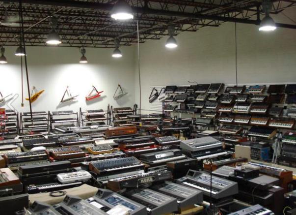
There is a tremendous variety of synths out there - both software and hardware. All shapes and sizes, with different feature sets, synthesis approaches and price tags from zero to many thousands of dollars.
The reason they all exist is that no one has yet created a synthesizer that can do it all - one which can replace them all. That's because such a synthesizer would need to be able to generate EVERY possible sound – whether that be imitating existing instruments or sound effects, or creating entirely new ones. The issues in trying to do this are firstly, no single existing synthesis technique can PRACTICALLY cover all the bases. Secondly, synthesis methods are continually evolving and new ones being discovered. Thirdly, although some types of synthesis can yield a wider sound palette than others, the subtleties are such that even two instruments implementing the SAME synthesis method will still have their own character and 'quirks' - even when programmed identically. In other words, on the tin they may 'do the same thing', and you may program them 'the same way', yet they STILL may end up sounding a little different.
What I'll present here is a kind of 'Programmer's Synthesis Notes' that should help you on your way to not only generating your first sounds from first principles, but in devising your own techniques with the building blocks and contributing to this fascinating field. It's a work in progress to which I will continuously add topics, so be sure to check back. All the waveform images here are the actual output of the algorithms implemented in PureBasic.
Sine Me Up
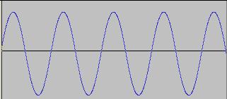
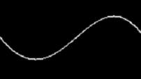
Let's start with the basic building block of sound - the sine wave.
| Hz | Frequency in Hz (cycles per second) |
|---|---|
| SR | Sampling Rate in Hz |
| O | Output |
| F | Frequency of wave (in Hz) |
| A | Amplitude of wave |
| T | Samples |
| L | Length of sound (in Samples) |
| Pi2 | 2*π = 6.28318530717958 |
The formula for a sine wave is:
O = A*(sin(F*T))
F determines the frequency of the waveform, as given by:
F = (Pi2*Hz)/SR
Hz is the actual frequency we want, but F is needed to produce a waveform at Hz frequency.
So, if we want to render 1000 samples of a 400Hz sinewave with Amplitude 1 (ie it should swing between 1 and -1) at a sampling rate of 44.1kHz, we would do this:
Hz = 400
L = 1000
A = 1
SR = 44100
F = (Pi2*Hz)/SR
For T = 0 to L
O = A*(sin(F*T))
Next T
O = A*(sin(F*T))
F determines the frequency of the waveform, as given by:
F = (Pi2*Hz)/SR
Hz is the actual frequency we want, but F is needed to produce a waveform at Hz frequency.
So, if we want to render 1000 samples of a 400Hz sinewave with Amplitude 1 (ie it should swing between 1 and -1) at a sampling rate of 44.1kHz, we would do this:
Hz = 400
L = 1000
A = 1
SR = 44100
F = (Pi2*Hz)/SR
For T = 0 to L
O = A*(sin(F*T))
Next T
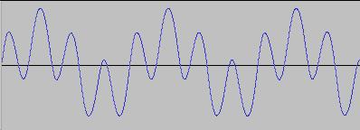
In Additive synthesis, we simply add together sine waves of different frequencies to create a sound. Let us say we have two sinewaves: O1 at 400 Hz, and O2 at 800 Hz. The additive waveform is then:
O3 = (O1 + O2)/2
Since we are taking the maximum Amplitude to be 1 here, and we want O3 to be no greater than this, we divide the result by the number of waves being added together - in this case 2.
O3 = (O1 + O2)/2
Since we are taking the maximum Amplitude to be 1 here, and we want O3 to be no greater than this, we divide the result by the number of waves being added together - in this case 2.
This principle is demonstrated by the sound engine of Paint2Sound.
Phase Value
Any sound can theoretically be created through the addition of sine waves of different frequencies, but not only do computers struggle in dynamically adding thousands of such waves together to generate a sound, it is difficult for a user to specify - or even know - what frequencies of waves to use, what their amplitudes should be and how to arrange them to obtain a desired sound. A more practical approach is to distort the sine waves, which effectively allows us to 'create more from less'. In order to do this, we first re-express the calculation of our example sine wave like this:
Hz = 400
L = 1000
A = 1
SR = 44100
Phase_Add = F/SR
For T = 0 to L
O = A*(sin(Pi2*Phase))
Phase = Phase + Phase_Add
If Phase > 1 then Phase = Phase - 1
Next T
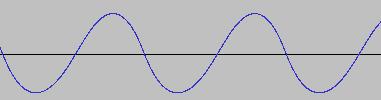
Here Phase is a variable which fluctuates between 0 and 1, and the Phase_Add increment determines the frequency of the sine wave. We can shift where the wave starts from in its cycle, by specifying the starting value of Phase as something other than 0. For example, if we set Phase = 0.25 before entering the For loop, the sine wave begins its journey from its maximum amplitude. The beauty of this new formula for generating a sine wave is that it allows us to manipulate the Phase in such a way that it forces a different waveform. Two of the foundation waveforms of subtractive synthesis (in which a waveform high in harmonic content is passed through a filter to selectively remove harmonics) are sawtooth and square waves. We can force such waveforms from our new sine wave formula, like so:
Hz = 400
L = 1000
A = 1
SR = 44100
Phase_Add = F/SR
For T = 0 to L
O = A*(sin(Pi2*PD(Phase)))
Phase = Phase + Phase_Add
If Phase > 1 then Phase = Phase - 1
Next T
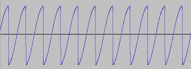
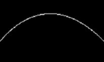
PD(Phase) is calling a function which distorts the Phase and causes O to trace a different waveform. Here is what PD(Phase) can look like to produce Saw and Square waves respectively:
Procedure PD(Ph)
;Saw wave
If Ph < 0.5
ProcedureReturn 0.35 * Sin(Ph)
Else
ProcedureReturn (0.35 * Sin(1 - Ph)) + 0.5
EndIf
EndProcedure
Hz = 400
L = 1000
A = 1
SR = 44100
Phase_Add = F/SR
For T = 0 to L
O = A*(sin(Pi2*Phase))
Phase = Phase + Phase_Add
If Phase > 1 then Phase = Phase - 1
Next T
Here Phase is a variable which fluctuates between 0 and 1, and the Phase_Add increment determines the frequency of the sine wave. We can shift where the wave starts from in its cycle, by specifying the starting value of Phase as something other than 0. For example, if we set Phase = 0.25 before entering the For loop, the sine wave begins its journey from its maximum amplitude. The beauty of this new formula for generating a sine wave is that it allows us to manipulate the Phase in such a way that it forces a different waveform. Two of the foundation waveforms of subtractive synthesis (in which a waveform high in harmonic content is passed through a filter to selectively remove harmonics) are sawtooth and square waves. We can force such waveforms from our new sine wave formula, like so:
Hz = 400
L = 1000
A = 1
SR = 44100
Phase_Add = F/SR
For T = 0 to L
O = A*(sin(Pi2*PD(Phase)))
Phase = Phase + Phase_Add
If Phase > 1 then Phase = Phase - 1
Next T
PD(Phase) is calling a function which distorts the Phase and causes O to trace a different waveform. Here is what PD(Phase) can look like to produce Saw and Square waves respectively:
Procedure PD(Ph)
;Saw wave
If Ph < 0.5
ProcedureReturn 0.35 * Sin(Ph)
Else
ProcedureReturn (0.35 * Sin(1 - Ph)) + 0.5
EndIf
EndProcedure
Procedure PD(Ph)
;Square wave
If Ph < 0.5
ProcedureReturn 0.25
Else
ProcedureReturn 0.75
EndIf
EndProcedure
;Square wave
If Ph < 0.5
ProcedureReturn 0.25
Else
ProcedureReturn 0.75
EndIf
EndProcedure

We can of course generalize the function for a Square wave, to produce a Rectangular (Pulse) wave, where a Square wave is simply a special case with a duty cycle of 50%. As so:
Procedure PD(Ph)
;Pulse wave
If Ph < PW
ProcedureReturn 0.25
Else
ProcedureReturn 0.75
EndIf
EndProcedure
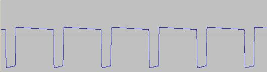
Where 0<PW<1, and a Square wave results when PW = 0.5. Here is a Pulse wave with PW = 0.2:
Procedure PD(Ph)
;Pulse wave
If Ph < PW
ProcedureReturn 0.25
Else
ProcedureReturn 0.75
EndIf
EndProcedure
Where 0<PW<1, and a Square wave results when PW = 0.5. Here is a Pulse wave with PW = 0.2:
The waveforms produced by these Phase Distortion functions need not be static. There are various ways the shape can by dynamically changed. For example, with reference to the Pulse function above, PW can be varied by an ADSR envelope generator or LFO. We can also morph between Phase Distortion functions; the following one for example will swing the output between a Sine and Square wave:
Procedure PD(Ph)
;morph between Sine and Square wave
;calculate a Square wave:
If Ph < 0.5
Q = 0.25
Else
Q = 0.75
EndIf
;a sine wave is simply:
S = Ph
;swing between the two according to another value z, where 0<z<1:
ProcecureReturn z*Q + (1-z)*S
EndProcedure
Once again, a LFO or ADSR envelope generator can be used to vary z. At z=0, O is a full Sine wave, and at z=1, it is a full Square wave. But there's no reason why we should restrict ourselves to reproducing 'traditional' synthesizer waveforms. The following function for example will produce a variety of waveforms for us:
Procedure PD(Ph)
;flexiwarper
If Ph<d
ProcedureReturn (v*Ph)/d
Else
ProcedureReturn (1-v)*((Ph-d)/(1-d)) + v
EndProcedure
Where 0<d<1. As d and v are varied (there are TWO independent dimensions to play with this time), a wide range of wave shapes are produced, from narrow impulses to full cycle sinusoids. When d=0.5 and v>1.5, formants are created, centred around harmonics of the fundamental frequency. This technique is implemented in Phase-Warper:
Procedure PD(Ph)
;morph between Sine and Square wave
;calculate a Square wave:
If Ph < 0.5
Q = 0.25
Else
Q = 0.75
EndIf
;a sine wave is simply:
S = Ph
;swing between the two according to another value z, where 0<z<1:
ProcecureReturn z*Q + (1-z)*S
EndProcedure
Once again, a LFO or ADSR envelope generator can be used to vary z. At z=0, O is a full Sine wave, and at z=1, it is a full Square wave. But there's no reason why we should restrict ourselves to reproducing 'traditional' synthesizer waveforms. The following function for example will produce a variety of waveforms for us:
Procedure PD(Ph)
;flexiwarper
If Ph<d
ProcedureReturn (v*Ph)/d
Else
ProcedureReturn (1-v)*((Ph-d)/(1-d)) + v
EndProcedure
Where 0<d<1. As d and v are varied (there are TWO independent dimensions to play with this time), a wide range of wave shapes are produced, from narrow impulses to full cycle sinusoids. When d=0.5 and v>1.5, formants are created, centred around harmonics of the fundamental frequency. This technique is implemented in Phase-Warper:
Also, fluctuating the phase of a sine oscillator with a relatively simple function can sometimes yield extremely complex and chaotic results, as demonstrated to good effect by Chaosurus.
These examples should go some way towards illustrating the 'Power Of The Phase', and plenty of scope remains in exploring new Phase Distortion algorithms.
These examples should go some way towards illustrating the 'Power Of The Phase', and plenty of scope remains in exploring new Phase Distortion algorithms.
Bit By Bit
Another way to distort a sine wave into more complex shapes is first to convert each of its sample values into an integer that can be represented on the bits of one byte, then directly manipulate those bits like shift them, rotate them, flip them, re-arrange them and so on, and finally convert the integer value represented by the new bit pattern back into a sample value to output. This is explored in a lot more detail on the Bit Twiddler page.
Suffice it to say this technique is capable of producing a wide range of weird and wonderful waveforms like these:
Suffice it to say this technique is capable of producing a wide range of weird and wonderful waveforms like these:
|
|
|
Pierre Bézier
Now the rules might say this is cheating, but yet another way of distorting a sine wave is not to start with a true sine wave at all, but a bezier curve (those things used for drawing paths in computer aided design and graphics programs), and adjust it to LOOK like a sine wave - it won't be exact, but can come close.
A bezier curve runs from a start point to an end point, with the curvature influenced by one or more intermediate control points. The cubic bezier function here is for example what's used in Quad-Klanger - we simply adjust the positions in this function of the initial and final (x,y) co-ordinates (these remain fixed), and the two control points then allow us to pull the curve into a sine-like waveform. Once we have this, we just move the control points around to warp this pseudo-sine wave into other shapes. So, here we have an alternative way of easily obtaining a variety of wave shapes from a sine - or more correctly - an approximate sine!
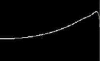
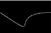
In each of the following pair of screenshots, the image on the left is that of a Bezier curve shaped in Quad-Klanger, and on the right is a capture of the corresponding sound output:
A bezier curve runs from a start point to an end point, with the curvature influenced by one or more intermediate control points. The cubic bezier function here is for example what's used in Quad-Klanger - we simply adjust the positions in this function of the initial and final (x,y) co-ordinates (these remain fixed), and the two control points then allow us to pull the curve into a sine-like waveform. Once we have this, we just move the control points around to warp this pseudo-sine wave into other shapes. So, here we have an alternative way of easily obtaining a variety of wave shapes from a sine - or more correctly - an approximate sine!
In each of the following pair of screenshots, the image on the left is that of a Bezier curve shaped in Quad-Klanger, and on the right is a capture of the corresponding sound output:
|
|
|
|
|
|
|
|
Sine Out
To 'round out' our discussion, a couple more techniques for turning sine (or 'sine-ish') to 'something other than sine' are worth mentioning:
We can have a polar equation represent the Phase. The polar coordinate system traces points on the plane (r, θ) where r is the distance from the origin and the angle θ is from the positive x-axis, measured counter-clockwise. The polar coordinates (r, θ) of a point are related to the x and y coordinates of a point, and we can have the y coordinate value sweep out our waveform as θ rotates between 0 and 2π. Polar equations can trace a variety of interesting shapes (the simplest being a circle which sweeps out a sine wave) and the technique is described in more detail on the SuperSoundShaper page.
A sine-like wave can also be a 'special case' of the dynamics of coupled non-linear differential equations which model a variety of 'real world' phenomena (certain coefficient values can produce such a waveform, but what we are typically interested in is the more 'exotic' wave shapes that other coefficient values yield). This is explored in more detail on the NeuronoiZ page.
Take Two
As we've discussed, we would need a bucket load of oscillators if we want to create very complex sounds and if we want to do this by just adding their outputs. But we can do other things which will give us several waveforms with just two oscillators, and with little computation. One such technique is Frequency Modulation. Given two oscillators, simple FM synthesis would look like this:
For T = 0 to L
O1 = A1*(sin(Pi2*PD(Phase1)))
O2 = A2*sin((Pi2*PD(Phase2))+FI*O1)
Phase1 = Phase1 + Phase_Add1
Phase2 = Phase2 + Phase_Add2
If Phase1 > 1 then Phase1 = Phase1 - 1
If Phase2 > 1 then Phase2 = Phase2 - 1
Next T
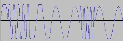
Where O2 is the Frequency Modulated output of the second oscillator and FI is a Feed In factor (typically 0<FI<50), which determines the 'intensity' of the modulation. The interaction of the two oscillators in this manner produces many sidebands in the O2 output. If the frequency of one of the oscillators is a multiple of the other, a harmonic timbre (instrumental sound) is produced, otherwise inharmonic timbres are created (like metallic/percussion sounds). The following shows O2 when FI = 5, and the PD(Phase) functions for both oscillators are set to produce sine waves:
For T = 0 to L
O1 = A1*(sin(Pi2*PD(Phase1)))
O2 = A2*sin((Pi2*PD(Phase2))+FI*O1)
Phase1 = Phase1 + Phase_Add1
Phase2 = Phase2 + Phase_Add2
If Phase1 > 1 then Phase1 = Phase1 - 1
If Phase2 > 1 then Phase2 = Phase2 - 1
Next T
Where O2 is the Frequency Modulated output of the second oscillator and FI is a Feed In factor (typically 0<FI<50), which determines the 'intensity' of the modulation. The interaction of the two oscillators in this manner produces many sidebands in the O2 output. If the frequency of one of the oscillators is a multiple of the other, a harmonic timbre (instrumental sound) is produced, otherwise inharmonic timbres are created (like metallic/percussion sounds). The following shows O2 when FI = 5, and the PD(Phase) functions for both oscillators are set to produce sine waves:
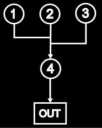
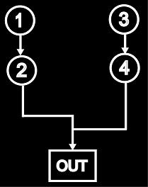
If we have more than two oscillators, we can add and FM them in various combinations to create complex sounds (what Yamaha called 'algorithms' when they implemented FM in their DX line of synths). For example, the following diagrams show only two possible combinations with four oscillators - or 'operators' in Yamaha-speak. (We observe though that with any combination, there is still only ever one modulation frequency applied to a waveform at once. This is where Bezier Curve synthesis introduced earlier can add a different flavour, since in that case modulation of the two control points independently in the x and y directions allows four separate modulation frequencies to be applied simultaneously).
|
1 + 2 + 3 -> X (Add the waveforms)
X -> 4 -> OUT (FM. X is modulating oscillator 4) |
|
1 -> 2 -> X (FM. Oscillator 1 is modulating oscillator 2)
3 -> 4 -> Y (FM. Oscillator 3 is modulating oscillator 4) X + Y -> OUT (Add the waveforms) |
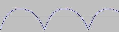
Actually, even if we only have one sine oscillator at our disposal we can still borrow something from the two oscillator FM technique to easily produce rich timbres with the one oscillator. What we do is that instead of feeding back one oscillator into the other, we use the single oscillator as part of its own calculation for feedback. In other words, we make the sine wave modulate itself by mixing back some of the output. Like this:
For T = 0 to L
O = A*sin((Pi2*PD(Phase))+FB*O)
Phase = Phase + Phase_Add
If Phase > 1 then Phase = Phase - 1
Next T
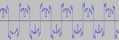
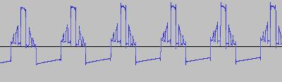
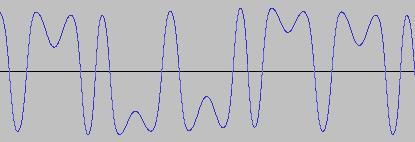
Where PD(Phase) is set to produce a sine wave, and the Feedback constant FB is just like the Feed In constant FI in the two oscillator FM case. If we make 0<FB<50, the lower FB values produce a distorted sine wave, and as FB increases, the waveform looks (and sounds) more and more like white noise. This is what the output O looks like when FB = 1.2:
For T = 0 to L
O = A*sin((Pi2*PD(Phase))+FB*O)
Phase = Phase + Phase_Add
If Phase > 1 then Phase = Phase - 1
Next T
Where PD(Phase) is set to produce a sine wave, and the Feedback constant FB is just like the Feed In constant FI in the two oscillator FM case. If we make 0<FB<50, the lower FB values produce a distorted sine wave, and as FB increases, the waveform looks (and sounds) more and more like white noise. This is what the output O looks like when FB = 1.2:
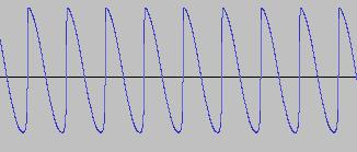
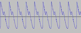
When FB = 2:
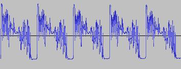
When FB = 5:
Given a couple of oscillators we can also synchronize one to the other so that each time the 'master' oscillator completes a cycle, it resets the Phase of the second oscillator. If the 'master' frequency is lower than the 'slave' frequency, changing the pitch of the slave changes the harmonic content of the output, but the pitch of the output remains that of the master. Thus if we have two oscillators generating waveforms of different frequency like so:
For T = 0 to L
O1 = A1*(sin(Pi2*PD(Phase1)))
O2 = A2*(sin(Pi2*PD(Phase2)))
Phase1 = Phase1 + Phase_Add1
Phase2 = Phase2 + Phase_Add2
If Phase1 > 1 then Phase1 = Phase1 - 1
If Phase2 > 1 then Phase2 = Phase2 - 1
Next T
Then a hard-sync of the second oscillator to the first would be achieved like this:
For T = 0 to L
O1 = A1*(sin(Pi2*PD(Phase1)))
O2 = A2*(sin(Pi2*PD(Phase2)))
Phase1 = Phase1 + Phase_Add1
Phase2 = Phase2 + Phase_Add2
If Phase1 > 1 then
Phase1 = Phase1 - 1
Phase2=0
EndIf
If Phase2 > 1 then
Phase2 = Phase2 - 1
EndIf
Next T
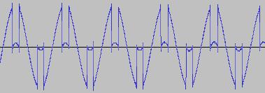
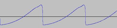
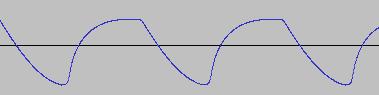
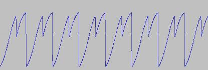
The following shows the output O2 of oscillator 2, where PD(Phase2) is set to produce a sawtooth wave and oscillator 2 is synced to oscillator 1 using the above method:
For T = 0 to L
O1 = A1*(sin(Pi2*PD(Phase1)))
O2 = A2*(sin(Pi2*PD(Phase2)))
Phase1 = Phase1 + Phase_Add1
Phase2 = Phase2 + Phase_Add2
If Phase1 > 1 then Phase1 = Phase1 - 1
If Phase2 > 1 then Phase2 = Phase2 - 1
Next T
Then a hard-sync of the second oscillator to the first would be achieved like this:
For T = 0 to L
O1 = A1*(sin(Pi2*PD(Phase1)))
O2 = A2*(sin(Pi2*PD(Phase2)))
Phase1 = Phase1 + Phase_Add1
Phase2 = Phase2 + Phase_Add2
If Phase1 > 1 then
Phase1 = Phase1 - 1
Phase2=0
EndIf
If Phase2 > 1 then
Phase2 = Phase2 - 1
EndIf
Next T
The following shows the output O2 of oscillator 2, where PD(Phase2) is set to produce a sawtooth wave and oscillator 2 is synced to oscillator 1 using the above method:
What else? Well, we can multiply the output of the two oscillators, in which case we get Amplitude Modulation:
For T = 0 to L
O1 = sin(Pi2*PD(Phase1))
O2 = sin(Pi2*PD(Phase2))
Out = (A2+A1*O1)*O2
Phase1 = Phase1 + Phase_Add1
Phase2 = Phase2 + Phase_Add2
If Phase1 > 1 then Phase1 = Phase1 - 1
If Phase2 > 1 then Phase2 = Phase2 - 1
Next T
A1 and A2 are the scaling coefficients in the range [0,1]. If A1 = 0, there is no modulation and the output is simply the scaled output of oscillator 2. If A2 = 0 and A1>0, sidebands are generated centred around the frequency of O2 (this form of AM is called Ring Modulation). A2>0 produces various forms of 'suppressed carrier' AM. A2 = 1 and A1>0 generates 'double sideband full carrier AM'. In practice, Out should be scaled to prevent clipping. Best results with AM are achieved when PD(Phase1) and PD(Phase2) are set to produce waveforms OTHER than sine waves. But even with sine waves it can be interesting feeding an Amplitude Modulated signal back to the amplitude input of the oscillator (in other words using the output of the oscillator as its modulator). So two sinusoid feedback AM oscillators might look like this:
For T = 0 to L
O1 = (1+A1*O1)*sin(Pi2*PD(Phase1))
O2 = (1+A2*O2)*sin(Pi2*PD(Phase2))
Phase1 = Phase1 + Phase_Add1
Phase2 = Phase2 + Phase_Add2
If Phase1 > 1 then Phase1 = Phase1 - 1
If Phase2 > 1 then Phase2 = Phase2 - 1
Next T
For the overall output we could then add O1 and O2, or again AM them together, and so on.
For T = 0 to L
O1 = sin(Pi2*PD(Phase1))
O2 = sin(Pi2*PD(Phase2))
Out = (A2+A1*O1)*O2
Phase1 = Phase1 + Phase_Add1
Phase2 = Phase2 + Phase_Add2
If Phase1 > 1 then Phase1 = Phase1 - 1
If Phase2 > 1 then Phase2 = Phase2 - 1
Next T
A1 and A2 are the scaling coefficients in the range [0,1]. If A1 = 0, there is no modulation and the output is simply the scaled output of oscillator 2. If A2 = 0 and A1>0, sidebands are generated centred around the frequency of O2 (this form of AM is called Ring Modulation). A2>0 produces various forms of 'suppressed carrier' AM. A2 = 1 and A1>0 generates 'double sideband full carrier AM'. In practice, Out should be scaled to prevent clipping. Best results with AM are achieved when PD(Phase1) and PD(Phase2) are set to produce waveforms OTHER than sine waves. But even with sine waves it can be interesting feeding an Amplitude Modulated signal back to the amplitude input of the oscillator (in other words using the output of the oscillator as its modulator). So two sinusoid feedback AM oscillators might look like this:
For T = 0 to L
O1 = (1+A1*O1)*sin(Pi2*PD(Phase1))
O2 = (1+A2*O2)*sin(Pi2*PD(Phase2))
Phase1 = Phase1 + Phase_Add1
Phase2 = Phase2 + Phase_Add2
If Phase1 > 1 then Phase1 = Phase1 - 1
If Phase2 > 1 then Phase2 = Phase2 - 1
Next T
For the overall output we could then add O1 and O2, or again AM them together, and so on.
